So we got forward mode, essentially free. Sweet.
However, if you look into the code for Jet, what you'll see, is that it's tracking the gradient of every partial derivative, through every calculation. If you were to have a large number of input dimensions (e.g. training a neural net) this calculation gets expensive. I believe it to be O(n).
The motivation for reverse mode differentiation, is that it is O(1).
The implementation is fascinating from both a maths and implementation perspective. The reverse mode AD algorithm uses some cunning mathematics (not described here) and required you to build a directed (acyclic) graph of the calculation. Gradients are then pushed "backward" through the graph. An example
import spire._
import spire.math._
import spire.implicits.*
import _root_.algebra.ring.Field
import spire.algebra.Trig
import vecxt.all.*
import vecxt.BoundsCheck.DoBoundsCheck.yes
import spire.math.Jet.*
import io.github.quafadas.inspireRAD.*
import io.github.quafadas.inspireRAD.TejVDoubleAlgebra.*
import io.github.quafadas.inspireRAD.TejVDoubleAlgebra.ShowDetails.given

given graph: TejVGraph[Double] = TejVGraph[Double]()

val data = Matrix.fromRows(
  Array(1.0, 2.0),
  Array(-1.0, -2),
  Array(4.0, 5.0)
).tej
// data: TejV[Matrix, Double] = TejV(value = vecxt.matrix$Matrix@78be4cd)

val weights = Matrix.fromColumns(Array(0.1, 0.2), Array(0.05, 0.1)).tej
// weights: TejV[Matrix, Double] = TejV(value = vecxt.matrix$Matrix@7ab7ac73)

val probits = (data @@ weights).exp.normaliseRowsL1
// probits: TejV[[A >: Nothing <: Any] =>> Matrix[A], Double] = TejV(
//   value = vecxt.matrix$Matrix@7857fe70
// )
val selected = probits(Array((0,0), (1,1), (2, 0))).mapRowsToScalar(ReductionOps.Sum).log.mean
// selected: TejV[[T >: Nothing <: Any] =>> Scalar[T], Double] = TejV(
//   value = Scalar(scalar = -0.5183549628810483)
// )

val loss = selected * -1.0.tej
// loss: TejV[[T >: Nothing <: Any] =>> Scalar[T], Double] = TejV(
//   value = Scalar(scalar = 0.5183549628810483)
// )

loss.backward((weights = weights))
// res0: NamedTuple[Tuple1["weights"], *:[Matrix[Double], EmptyTuple]] = Tuple1(
//   _1 = vecxt.matrix$Matrix@37965b64
// )
traced.backward(weights) does the backward pass, and returns a named tuple of the gradient of the loss variable with respect to the input nodes, in this case "weights".
It is possible to inspect the calculation graph which is carried around in side the TejDim given.
graph.dag.toGraphviz will return a string representation of the graph. If you paste the output of the calculation graph into an online graphviz editor, you'll see something like this.
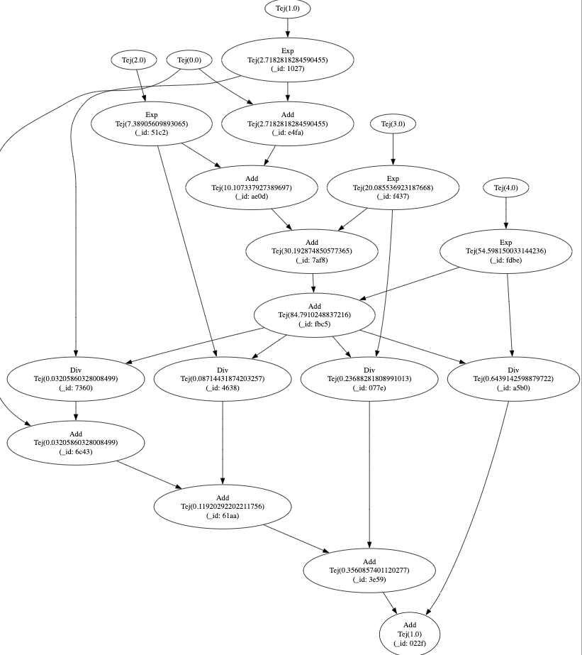
To do it, it navigates the graph in reverse topological order, propagating its gradient to its child nodes in accordance with the chain rule. Hopefully.